Hazard Package
Hazard Function Technology
Time-related events are some of the most important outcomes of medical procedures and the life-history of machines. The "raw data" for such events is the time interval between the defined "time zero" (t=0) and the occurrence of the event. The distribution of a collection of these time intervals can be viewed as a cumulative distribution table or graph. However, the complement of the cumulative distribution is commonly displayed as a survivorship function.
Another way to visualize the intervals is as a histogram or probability density function; however, because the fundamental questions about these intervals relate to some biologic or natural phenomenon across time, the more natural domain for study is; the rate of occurrence.
The rate of occurrence of a time-related event is known as the hazard function or "force of mortality." In financial circles, it is the inverse of Mills ratio. The methodology embodied in the hazard function analysis is applicable to any positively distributed variable.
The nature of living things and real machines is such that lifetimes (or other time-related events) often lead to rather simple, low-order distributions. For this reason, we believed that low-order, parametric characterization of the distribution can be accomplished.
The parametric approach taken in the hazard procedures developed in the early 1980s at the University of Alabama at Birmingham was a decompositional approach. The distribution of intervals is viewed as consisting of one or more overlapping "phases" (early, constant, and late) additive in hazard (competing risks). A generic functional form is utilized for the phases that can be simplified into a large number of hierarchically nested forms.
Each phase is scaled by a log-linear function of concomitant information. This allows the model to be non-proportional in hazards, an assumption often made, but often unrealistic.
Finally, the hazard model has been enriched in 3 ways.
- Because the intervals may not be known completely (incomplete, censored data), right censoring, left censoring, and interval censoring are incorporated into the procedure.
- Second, the events considered may be repeating. This automatically accommodates a wide class of time-varying co-variables, that can be considered to change at specific intervals.
- Third, the event may be weighted on a positive scale (such as cost). Thus, the procedure, at its most complex, can accommodate time-related repeating cost data, with time-varying co-variables, and a non-proportional hazard structure.
Documentation
Overview of Procedures: Parametric Analysis of Time-Related Events.
This document contains various documentation related to the Hazard in assorted formats. Two SAS-interfaced procedures, PROC HAZARD and PROC HAZPRED, are described. These procedures constitute an analysis system for generalized completely parametric censored-data analysis and display. They utilize the scheme of decomposition of the distribution of times to an event (or of any positive variable) into up to 3 overlapping phases of hazard (competing risks), each phase scaled by a parametric function of concomitant variables. The equations and general methods for using the procedures are given in this overview, while details of syntax are given in the subsequent two documents specifying the procedures. View document (PDF)
The HAZARD Procedure
PROC HAZARD is a procedure for parametric analysis of time-related events. However, you may use it to model arbitrary distributions of positive valued variables substituted for the TIME variable name. A detailed description of the model has been given in the overview document, Parametric Analysis of Time-Related Events: Overview of Procedures (PDF).
The HAZPRED Procedure
PROC HAZPRED is a procedure for calculation of time-related estimates (predictions) from a parametric equation previously established by PROC HAZARD. View document (PDF)
For questions or to request additional download formats, please contact us at [email protected]
The Hazard Package Downloads
The Hazard Package is a set of programs for the analysis of hazard functions. Originally developed at the University of Alabama at Birmingham, the package is currently being maintained and developed at Cleveland Clinic. The code is being made available in both source code and a small set of pre-compiled packages.
The Hazard package is designed to run within SAS®. Macros and installation instructions are included to integrate the package into your SAS® installation.
Binary Distributions
You can download a precompiled version of the Hazard package through the following links. The programs included in this package have been successfully compiled, linked, and executed on the following platforms:
- IBM AIX
- SUN Solaris 5.6
- Microsoft Windows (2000/NT)
- Microsoft Windows (95/98/ME)
To install the binary package simply unpack the distribution file in an application parent directory (i.e. /usr/local or c:\). A distribution file will create the following directory structure:
- hazard
HAZARD The hazard root - hazard/bin
HAZAPPS The executable directory - hazard/doc
Documentation for the system - hazard/examples
HZEXAMPLES Example programs - hazard/examples/data
Example data - hazard/examples/output
Results that we got from the example programs. - hazard/examples/sasest
SAS estimate data files - hazard/examples/sasest/ihd
A SAS estimate data file - hazard/macros
MACROS The utility macro directory.
Then proceed the appropriate installation instructions for MS Windows or Unix based platforms.
We have no way of testing these programs, or constructing specific installation instructions, for other systems. However, we hope that these guidelines below help you decide what should be done on your own system. We appreciate any feedback regarding the process you use to install HAZARD. This will enable us to provide that information to others, so that their task will possibly be easier. We would also welcome contributions of packaged executable kits, compiled for different platforms.
Source Code Distribution
Our C code has been ported to other systems, and appears to compile and run with no problems. Nevertheless, even in the world of 'standard' C, there may be unexpected incompatibilities between our systems, particularly with regard to mathematical precision and library function parameters. If you encounter such problems, please let us know. We can attempt to work around them and make adjustments so that future versions will work on yours and similar systems without special effort.
Requirements
The HAZARD package is written entirely in ANSI standard C, and uses lex and yacc for parsing its input commands. You must have equivalent compilers installed on your system before attempting to install HAZARD. Fortunately, all are freely available on the Internet, thanks to the GNU project.
You can download GCC, a C / C++ compiler, from the GNU Compiler Collection.
Once you have compiled GCC, you can download the Flex lex program and Bison, the parser compiler.
If you would like to compile the program on the Windows platform, we suggest you use the tools from the Cygwin project. This package includes all the tools required to compile the HAZARD system.
Then, download the hazard source distribution file.
- UNIX gzipped tar file
- Now proceed to the installation instructions by clicking on the "Intallation" tab at the top.
The Hazard Package Examples
Analysis Examples
Datasets
AVC
The first example is a short (n=310) data set with a few variables of the many studied is included as '!HZEXAMPLES/data/avc'. (The lesion is a form of congenital heart disease known as atrioventricular septal defects, or atrioventricular (AV) canal. The entire spectrum of lesions is included from partial through intermediate to complete forms, in that with this many cases, the data looked indeed like a spectrum, not 3 isolated forms.) The follow-up is such that at present, there are two hazard phases: the early phase after the operation, and a constant hazard phase. As time goes on, the hazard will again rise, if for no other reason - aging. Duration of follow-up time, as well as the actual distribution of events, will dictate how many phases of hazard are found (NOTE: we use "phases" as a more understandable term to clinicians than "mixture distribution components").
TheAVC example dataset is stored in a file named !HZEXAMPLES/examples/data/avc.
Normally this would be a SAS data set, probably built from the raw data. For illustration, a few variables from a data set for repair of atrioventricular septal defects will be read from a "flat file."
OMC
For a complete change of pace, another data set is included that has within it a repeated event (thromboembolism) and an evaluation of the seriousness of the event. In hz.te123 we look at two ways of analyzing such data: straight repeated event methodology using longitudinal segmentation of the observation as described in the documentation and left censoring, and a modulated renewal process. When the latter is valid, it makes for a much more interpretable analysis, in my opinion. In hz.tm123, the event is analyzed as a weighted outcome variable, using the WEIGHT statement.
The OMC example dataset is stored in a file named $HZEXAMPLES/examples/data/omc.
CABGKUL
The CABGKUL example dataset is stored in a file named $HZEXAMPLES/examples/data/cabgkul.
Examples
ac.death.AVC.sas
Life Table for death after repair of atrioventricular septal defect
hz.death.AVC.sas
Determine Hazard Function for Death after repair of atrioventricular septal defects.
This job concentrates on determining the shaping parameter estimates for the overall (underlying) distribution of event. It is the major exercise that is different from Cox. It can be time-consuming at first, and has all the frustrations of nonlinear estimation.
The time for these exercises can vary from about five minutes to one hour. The non-parametric cumulative hazard function provides all the clues. Start with simple models and work up (because it is easy to get into an overdetermined state). The final models are rarely complex.
For example, an n=6000 coronary data set with 20 years follow-up will have all three phases present, with the hardest to fit late phase probably being a simple Weibul (late hazard=MUL*t**power), a constant hazard phase, and an early phase with M or NU likely simplifying to a constant (1 or 0). Do not use DELTA. However, note that sometimes the program will terminate abnormally, but with M or NU driven to near zero (E3 or E4 large negative numbers). This is a sign that you want to set NU or M to zero (M=0 FIXM, for example). When there are abnormal terminations, be sure that it is for something other than the computer trying to get close to minus infinity.
There are three different optimization algorithms available. In some problems, STEEPEST is needed, while in others QUASI works fine (sometimes in conjunction with STEEPEST), as does the Newton method. Sometimes the early phase will have some huge exponents--but there will be one of its three branches that will tame these exponents.
Read the documentation for support. If you are experiencing difficulty, reach out for assistance.
hz.deadp.KUL.sas
Survival after primary isolated CABG. Hazard function for death.
hz.te123.OMC.sas
Hazard function for repeated thromboembolic events.
hz.tm123.OMC.sas
Hazard function for permanent morbidity from thromboembolic events.
lg.death.AVC
Descriptive analysis of death after repair. Transformations of scale investigation.
hm.death.AVC
Multivariable analysis of death after repair
This job is an example of a multivariable analysis. The shaping parameters should be fixed during the process of obtaining the risk factors. The actual process of doing this is no more difficult than a logistic or Cox modeling effort. To make the job simpler, you are able to to a) exclude variables with an /E option but still look at their q-statistics for entry (equivalent to one Newton step), b) select variables with associated /S, and c) include variables with the /E option.
These are all directly associated with the variables, so you can keep your variables organized in their medically meaningful, and usually highly correlated, groups.
A stepwise procedure is provided, and is useful for a few steps (recommended for only 3-5 steps). It is not recommend to use automatic model building in absence of knowledge of the quality of each variable and the covariance structure. The only intellectual hurdle you must overcome is looking simultaneously at multiple hazard phases. However, this "buys" relaxation of proportional hazards assumptions, and takes into account (especially in surgical series) that some risk factors are strong early after operation, and much less so later.
The job also shows that as a final run, the best method is unfixing the shaping parameters, specifying all the estimates and making a final run. In theory, the shaping parameter values must change – by a small amount (that is, the average curve is not the same as setting all risk factors to zero). You may wish also to reexplore the early phase shaping parameters in the rare event that THALF gets much larger in this final step.
These are examples of exploring the strengths of risk factors either at a slice across time (hm.death.hm1) or across time (hm.death.hm1). The advantage of an all parametric model is that all you have to do is solve an equation.
hp.death.AVC.hm1
Multivariable analysis of death after repair of atrioventricular canals.
Exploration of strength of risk factors. A major strength of completely parametric models is that once parameter estimates are available, the resulting equation can be solved for any given set of risk factors. This permits, for example, solving the equation for the time-related survival of an individual patient by "plugging in" that patient's specific risk factors (patient-specific prediction).
In this example, we exploit the parametric model by exploring the shape of risk factors. Here, for a given set of risk factors, we compare survival in two otherwise similar patients, except that one has an additional major cardiac anomaly.
hp.death.AVC.hm2
- Multivariable analysis of death after repair
- Exploration of strength of risk factors.
- Display strength of date of repair in partial and complete forms of AV Canal
hs.death.AVC.hm1
Multivariable analysis of death after repair
Another strength of a completely parametric survival analysis is that the investigator can test the "goodness" of the model. Specifically, the theory of mixture distributions would indicate that if a survival curve (or death density function) is generated for each observation, the mean of these should be the overall survival curve. And for any subset of the data, such a subset mean should well fit the empiric survival curve (unless a risk factor has not been taken into account).
The theory of conservation of events also suggests that the sum of the cumulative hazard for each patient can predict the number of expected deaths, comparing this with the actual number. However, this requires caution as the cumulative hazard has a limitless upper bound. One could make the case for limiting any cumulative hazard estimate greater than 1.0 to that number.
As a type of internal validation, although the variable is in the model, partial and complete AV Canal can be predicted from the analysis, overlaying it with the nonparametric life table estimates to check out the model. Recall that there was concern that the log-likelihood was better when COM_IV was present in the constant hazard phase, but reliable estimates for that factor could not be obtained. This will help determine how inaccurate the results are by ignoring this factor in that phase.
In actual practice, there is a "setup" job that generates the curves for each patient in the data set and the cumulative hazard values. Once stored (often temporarily, for the data set size can be large), the data set can then be stratified to check accuracy using a separate job or set of jobs.
Notes
For practice fitting a variety of hazard shapes with up to three phases, you may now wish to explore the coronary artery bypass grafting data set. It contains the event death, return of angina, and reintervention. To get you started, hz.deadp.KUL is an annotated setup for the event death. You will want to start off with some actuarial estimates, as you did for the data set above, and work your way through all these events.
For practice at both fitting interesting hazard shapes, controversy as to what events should be "bundled" as a single event, and then exercising of the procedure's variable selection possibilities, a limited valve replacement data set ($HAZARD/examples/data/valves) is provided, along with a sample multivariable setup program hm.deadp.VALVES.
Since an important aspect of the model is exercising the resulting equations, we have included a number of plots (hp. jobs), as well, as a number of validation files (the hs jobs). These are internally commented.
Another use of predictions is for comparing alternative treatments from analyses of different data sets. One example of this is given in hp.death.COMPARISON, an example of comparison of PTCA, CABG and medical treatment.
Hazard Package Installation
This documents the steps required to install the Hazard package on your computer system. There are four basic steps to getting the system set up and running.
- Verify your SAS installation.
- Compile the source code.
- Install the binary executables.
- Setup the system and SAS environments.
Throughout the document, there are platform specific steps for Windows or UNIX. The UNIX experience is taken from the Solaris platform, but should be useful for all UNIX variants. The Windows experience is taken from Windows 2000, other versions are noted where possible.
Verify your SAS installation.
The Hazard package requires SAS for pre and post processing of data and result sets. Hazard has been successfully run on many versions of the SAS ® system. Hazard Version 4.1.x has been tested on SAS V 6.12 and V 8.x.
- You can test your version of SAS ® by simply executing the SAS command.
- UNIX: From the command line, issue the SAS command.
- Windows: From the start menu go to Programs and look for the SAS or SAS Institute program group and open the SAS program.
Compile the source code
If you downloaded the platform specific pre-compiled versions of the package, currently available for the Windows and Solaris platforms, you can skip to the next section.
If you are running a platform besides Windows or Solaris, you must compile your own executables from the source code distribution.
The HAZARD package written entirely in ANSI standard C, and uses lex and yacc for parsing its input commands. You must have equivalent compilers installed on your system before attempting to install HAZARD. Fortunately, all the tools required are available for many platforms from through the GNU project. The GCC C compiler system can be downloaded from gcc.gnu.org. You can also download the flex lexer and bison parser to perform the lex and yacc functions.
Compiling the source code has been greatly simplified in Version 4.1.x of the Hazard package. The autoconf package is now being used to automate the compile and install process. The steps are described in the INSTALL file in the root of the distribution. The basic steps are as follows:
- Decide where to install the executables. By default they will be installed in the /usr/local/hazard directory.
- Issue the ./configure command. If you want to move the installation directory, issue the command as configure --prefix=/install/directory/. An example install directory could be $HOME/hazard. The configure will build the make files required to compile the package. It will find required tools and environment to (hopefully) successfully build the system.
- Issue the make command to compile the code.
- Issue the make install command to completely install the package into your install directory.
UNIX:
If you have compiled the system on a platform besides Windows or Solaris, we would like to hear about your experiences. Please contact us. Please include the platform you are working on. If you would like to contribute a binary distribution kit, contact us for instructions on building the necessary files.
Windows:
A note about the Windows system. The Windows executables have been compiled from the same source code as the Unix versions. This was accomplished by using the CYGWIN tools. They are also freely available and can be downloaded from sources.redhat.com/cygwin. If you install the full distribution, you do not need to install any other tools. Once you install these tools, you can compile the sources into executables using the instructions given here.
The recommended installation directory under CYGWIN is c:\hazard. The configure command to install the program in this location is:
./configure --prefix=//c/hazard
Install the binary executables
Now that the programs have been compiled and linked into an executable form, you need to install the package. If you compiled your own executable, the make install command completes this process. You can then proceed to the setup section. From the Binary packages, follow the instructions for your specific platform.
UNIX:
You may need root access to complete the installation if you do not have permission to write to the installation directory.
Change to the parent of your installation directory and unpack the binary kit.
If you want the package installed in the hazard directory under your user home, cd to $HOME
Unpack the binary distribution.
Use the following command to unpack the distribution.
gzip -d < /path/to/distribution/hazard.PLATFORM.tar.gz | tar -xvf -
Windows:
Our team usesthe winzip package to unzip windows distributions. It is available at winzip.
Once you've installed Winzip, the Windows link will automatically launch the winzip application. You must "extract" the files to your installation directory. Because of some incompatibilities, you must install this in a root directory, such as c:\ directory.The distribution for any platform will create the hazard directory containing the standard hazard directory structure.
Setting up the system and SAS environments
The hazard package requires some environment variables to be set so that the macros that run the system know where to find the package directories. Different operating systems require different methods of setting these variables.
UNIX Setup
For Unix, the environment can be set in your startup files. If you are using ksh, bash or sh, use the export command from a .profile file.
export VARIABLE=value
for csh and it's variants use the setenv command in your .cshrc file
setenv VARIABLE value
If you need help setting these up correctly, contact your system administrator.
| VARIABLE | Recommended Variable Value | Description |
|---|---|---|
| Hazard Environment variables for Unix platforms | ||
| HAZARD | /usr/local/hazard or $HOME/hazard |
The root of the hazard installation |
| HAZAPPS | $HAZARD/bin | Executable files |
| HZEXAMPLES | $HAZARD/examples | Examples sas jobs and data sets |
| MACROS | $HAZARD/macros | Example SAS macros used by $HZEXAMPLE files |
Windows Setup
In Windows NT/2000/XP, From the Start menu choose Settings and Control Panels. Select the System control panel and go to the Advanced tab to set the Environment Variables....
Our team added the variables to the User variables for username using the New button in the upper section of the panel. If you have administration privilege, you can add them to the System variables so all users on the machine would not have to individually set their own environment.
In Windows 9X/ME, edit the Autoexec.bat file on your System Disk, usually the C: drive. Add a line of the following form for each environment variable:
set VARIABLE=value
The following variables should be defined. They are case sensitive.
| VARIABLE | Recommended Variable Value | Description |
|---|---|---|
| Hazard Environment variables for Windows platforms | ||
| TMPDIR | %TEMP% | The location the Hazard package stores temporary files. |
| HAZARD | c:\hazard | The root of the hazard installation |
| HAZAPPS | %HAZARD%\bin | Executable files |
| HZEXAMPLES | %HAZARD%\examples | Examples sas jobs and data sets |
| MACROS | %HAZARD%\macros | Example SAS macros used by %HZEXAMPLE% files |
You may need to restart you machine for the environment to be correctly setup.
You can now proceed to setting up your SAS environment.
SAS Setup
Finally, you need to SAS where to find the hazard and hazpred macros. Our versions of SAS the config file is named sasv8.cfg, you should find a similar file for your release of SAS.
UNIX:
On the unix platform, your personal version is located in your home directory ( ~/sasv?.cfg).
Our unix sasautos command look like this:
-sasautos ( '!SASROOT8/sasautos' '!HAZAPPS')
Windows:
On Windows, it is either in the c:\Program Files\Sas Institute\SAS\V8 directory or under your personal directory My Documents\My SAS Files\V8. The best way to find it is to do a search for sas*.cfg.
Edit your config file, and find the sasautos command and add the HAZAPPS environment variable to it. The ! character tells SAS to interpret the following name as an environment variable in a platform independent manner:
  /* Setup the SAS System autocall library definition */
-SET SASAUTOS  (
"!sasroot\core\sasmacro"
"!sasext0\graph\sasmacro"
"!sasext0\stat\sasmacro"
"!HAZAPPS"
)
On the Windows platform, add the following line to your sas config file
    /* Allow external commands to exit automatically */
-noxwait
By default, SAS causes externally run programs to automatically open a DOS command window. The default behavior of the window requires you to type exit at the command prompt to close each window. The -noxwait command changes the behavior so that the window will close automatically.
Testing Hazard Installation
The easiest way to test your Hazard installation is to run one of the Hazard example programs. Go to your !HZEXAMPLES directory and try running any/all of the example programs there. Documentation for the examples is located on the Examples page.
Further documentation of the hazard system is available on our Documentation page.
Contact Information
If you experience any difficulties with the installation or use of the HAZARD package, please contact us. The e-mail address is:
Or, our daytime phone number is 216.444.6712. We would appreciate any feedback about your positive and negative experiences with the package, as well.
The Hazard Package Macros
Included in '!HAZARD/macros' are also a number of MACROS that we have found useful.
bootstrap.hazard.sas
This macro implements for the hazard procedure bootstrap so-called "bagging" for variable selection. In its use, you will find that one of the most important features of the hazard variable selection is the RESTRICT statement. This allows you to identify closely linked variables (such as transformations of age, all variables related to patient size, and so forth), such that only one of each kind of variable is selected. Then, a count, either manually or by machine, can be made of the unique occurrences of variables.
chisqgf.sas
This is a Chi-square goodness-of-fit macro for comparing expected and observed events. It is called by hazard simulation jobs that we have designated as hs. in the examples.
deciles.hazard.sas
This macro sorts patients according to survival at a given point in time specified by the TIME= variable, and then examines expected and observed events within groups specified in number by the variable GROUPS=. This routine is useful in examining goodness-of-fit of multivariable models.
hazplot.sas
This macro is useful for determining the goodness-of-fit of your hazard function to the distribution of times to the event. We use the Kaplan-Meier method as an independent verification tool. The macro uses various transformations of scale to examine early and late time frames to indicate the correspondence between the parametric and nonparametric estimates. In addition, it compares observed and predicted numbers of deaths and the departure of these from one another. This is perhaps one of the best clues to lack of fit. It also indicates how many events are associated with each hazard phase so that you can avoid overdetermined models for each hazard phase.
kaplan.sas
This is a Kaplan-Meier life table analysis macro. Its only difference from most packaged Kaplan-Meier programs is in its calculation of confidence limits. The confidence limits used in this program are more exact than using the Greenwood formula.
logit.sas
This macro is one of two that is useful in calibrating continuous or ordinal variables to the event. It is useful for logistic regression as well as time-related analyses. It groups the patients in roughly equal numbers, examines the number of events, and displays these on the scale of risk that is appropriate for your analysis. Ideally, if there is an association between the variable and risk, it should align nicely and linearly on the scale of risk. We usually examine a number of different transformations of scale of the variable to see which aligns best.
logitgr.sas
This macro is similar to logit.sas except that, instead of dividing the groups into equal numbers, it divides the groups according to a specified grouping variable. Otherwise, the information is similar.
nelsonl.sas
This macro calculates nonparametric estimates for weighted repeated events according to the algorithm of Wayne Nelson. Unlike the Kaplan-Meier estimator, the Nelson estimator is defined in the cumulative hazard domain. The latter is particularly more suited to repeated events and specifically to weighted events (Nelson calls it the cost function).
nelsont.sas
This macro is a companion to kaplan.sas, with identical outputs and naming of variables. However, it calculates the life table by the method of Wayne Nelson, rather than by the method of Kaplan and Meier. In this method, an event that plunges the life table calculated by Kaplan and Meier to zero is instead set to a value commensurate with the cumulative hazard function.
plot.sas
This is a big macro for making "pretty plots". Because of changes made in some of the SAS® graph modules between version 6 and version 8, we do not recommend its use for version 8. We are working on redoing those sections of the macro that have been changed in version 8.
JPredictor
Java based temporal decomposition hazards nomograms. Graphical survival/hazard model patient prediction tool for surgical evaluation. View program
Power Calculations for Tests on a Vector of Binary Outcomes (MULTBINPOW)
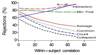
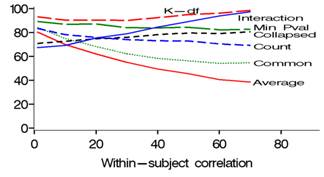
MULTBINPOW is a SAS simulation program which enables study planners to choose the most powerful among existing tests (see list below) when the outcome of interest is a composite binary-event endpoint. Mascha and Imrey (2010) compare the relative powers of standard and multivariate (GEE common effect and distinct effect) statistical tests for such situations. Relative power of the tests depends on several factors, including the size and variability of incidences and treatment effects across components, within-subject correlation, and whether larger or smaller components are affected by treatment. The average relative effect test (#5 below) is particularly useful in preventing the overall treatment effect estimate from being driven by components with the highest incidence, which is especially important in situations in which both incidences and treatment effects vary across components (e.g., Figs 1 and 2). This program allows the researcher to customize power calculations by choosing combination of these factors for a particular study, and then comparing power across the relevant statistical tests. Address questions or suggestions to [email protected].
Empirical power is calculated via simulations for 8 distinct statistical tests, each comparing 2 vectors of binary events (treatment versus control) under user-specified ranges of within-subject correlations, covariance structures, sample sizes and incidences.
Power is computed for the following tests:
- Collapsed composite of any-versus-none of the events
- Count of events within individual (Mann-Whitney and T-test)
- Minimum P-value test
- GEE common effect test (also called “global odds ratio” test).
- GEE average relative effect (distinct effects test, removes influence of high incident components)
- GEE K-df distinct effects test (analogous to Hotelling’s T2, not sensitive to direction)
- GEE covariance-weighted distinct effects test (usually very similar power to GEE common effect)
- GEE treatment-component interaction distinct effects test (whether treatment effect varies across vector)
Sample call:
For example, power calculations might be desired with the following specifications:
- Compare 2 vectors of 3 proportions each, with population proportions of
Treatment: (0.18 0.16 0.09) and Control: (0.20 0.20 0.15), with at alpha=0.05 - Weight outcomes for each group as 0.2, 0.4, 0.4, respectively.
- Assess power at within-subject correlations of 0.10, 0.30, 0.50 and N/group of 200, 400, 600.
- Produce 1000 simulations for each combination of within-subject correlation and N/group.
- Assume underlying exchangeable correlation for simulations, but use unstructured to analyze data.
- Summarize power in tables and graph; save individual simulation results in SAS dataset to be analyzed or appended to later.
MULTBINPOW would then be called as follows:
%let mypath=your directory to store simulation dataset results;
%inc "/your directory/multbinpow.sas";
%multbinpow(path=&mypath, reset=0, sims=1, summary=1, outdata=results, imlwt=0, startsim=1,
numsims=100,
pr_t= .18 .16 .09, pr_c= .20 .20 .15, rmin=10, rmax=50, rby=20,nmin=200,nmax=600,nby=200,
rmat=2, use_rmat=3, wt=.2 .4 .4, spar_ck=0, where=,simseed=1234, alpha=.05, listres=0, clearlog=1);
Additional options: increase the number of simulations without starting over; turn on the LISTRES option to see all analysis results for 1 or more simulations; assess the potential range of within-subject correlations for the given set of underlying proportions before running simulations.
For explanation of all options, see the header in the MULTBINPOW Program File or the README file.
Output:
The above call generates the following datasets, figure and output.
- Main results for each simulation run are saved to a SAS file with the user-specified filename, &outdata. This SAS dataset contains one observation for each simulation run for each specified combination of within-subject correlation and per-group sample size. Data for each simulation include the observed vectors of response proportions for treatment, control and overall, all parameter and test results, and a counter of simulation run (SIMI). Results are also saved to separate files particular to each specified combination of within-subject correlation and per-group sample size.
- A summary dataset named &outdata._sum is also created when summary=1 and makesum=1 are used. It has one record for each combination of NPER and RHO specified, and summary statistics for power, all relevant parameter estimates and standard errors, correlations, outcome vectors, etc.
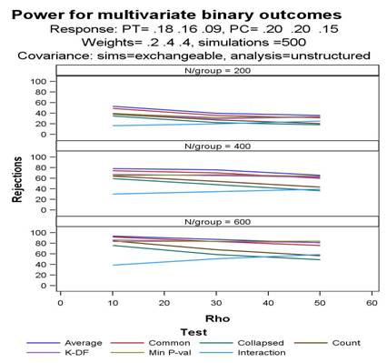
- Tabulated results. The generated output ( .lst file) gives the power for each test and summary statistics for the estimated vectors of proportions, working correlation matrix (partial results), and estimated treatment effects and standard errors for the main tests across the simulations. Tabulations are made using the dataset &outdata._sum. Default output for the above macro call is as follows:
Power calculations for multivariate binary outcomes based on 500 simulations
PT= .18 .16 .09, PC= .20 .20 .15 Component weights= .2 .4 .4 SASprogram =temp11
Covariance: simulation=exchangeable, analysis=unstructuredN/Group
200 400 600
Rho Rho Rho
0.100 0.300 0.500 0.100 0.300 0.500 0.100 0.300 0.500Mean Mean Mean Mean Mean Mean Mean Mean Mean
Number of components 3.00 3.00 3.00 3.00 3.00 3.00 3.00 3.00 3.00
Pc1 0.20 0.20 0.20 0.20 0.20 0.20 0.20 0.20 0.20
Pc2 0.20 0.20 0.20 0.20 0.20 0.20 0.20 0.20 0.20
Pc3 0.15 0.15 0.15 0.15 0.15 0.15 0.15 0.15 0.15
Pt1 0.18 0.18 0.18 0.18 0.18 0.18 0.18 0.18 0.18
Pt2 0.16 0.16 0.16 0.16 0.16 0.16 0.16 0.16 0.16
Pt3 0.09 0.09 0.09 0.09 0.09 0.09 0.09 0.09 0.09
GEE working corr(1,2) 0.08 0.25 0.41 0.08 0.25 0.41 0.08 0.25 0.42
GEE working corr(1,3) 0.06 0.19 0.32 0.06 0.19 0.32 0.06 0.19 0.32
Beta collapsed composite -0.32 -0.26 -0.23 -0.32 -0.28 -0.24 -0.32 -0.27 -0.23
SE(B) collapsed composite 0.21 0.21 0.22 0.15 0.15 0.16 0.12 0.12 0.13
Beta common effect -0.34 -0.32 -0.33 -0.33 -0.35 -0.34 -0.34 -0.34 -0.34
SE(B) common effect 0.18 0.20 0.22 0.13 0.14 0.16 0.10 0.12 0.13
Beta average relative effect -0.37 -0.36 -0.37 -0.36 -0.38 -0.37 -0.37 -0.37 -0.37
SE(B) avg rel effect 0.19 0.21 0.22 0.13 0.14 0.16 0.11 0.12 0.13
Pow collapsed comp (Wald) 0.35 0.22 0.18 0.60 0.48 0.37 0.76 0.59 0.49
Pow Count (MW) 0.38 0.28 0.20 0.64 0.54 0.43 0.85 0.68 0.57
Pow Count (pooled t) 0.42 0.29 0.25 0.67 0.62 0.51 0.87 0.77 0.67
Pow common effect (Wald) 0.49 0.36 0.31 0.74 0.70 0.60 0.92 0.83 0.76
Pow avg rel effect (Wald) 0.53 0.40 0.36 0.78 0.76 0.66 0.94 0.87 0.81
Pow avg rel effect(Score) 0.54 0.40 0.36 0.78 0.76 0.66 0.94 0.87 0.81
Pow K-df distinct(Wald) 0.40 0.30 0.33 0.67 0.65 0.62 0.86 0.83 0.82
Pow min bootstrap P-val 0.39 0.32 0.34 0.65 0.67 0.64 0.84 0.84 0.84
Pow TX-component interaction
(Score) 0.17 0.20 0.25 0.30 0.35 0.39 0.39 0.51 0.59 Graphs of power versus within-subject correlation by test are saved to a user-specified file, as below. Graphs are made using the dataset &figdata, with variables nper, r, meanvar (power) and test.
![]()
Download program. Download the MULTBINPOW program here. Runtimes vary proportional to the specified sample sizes and number of scenarios chosen. Proc IML is invoked only for test #7 listed above, which substantially increases runtime. To not include that test, use option IMLWT=0.
References
Mascha EJ, Imrey PB: Factors affecting power of tests for multiple binary outcomes. Statistics in Medicine 2010; 29: 2890-2904.
Oman Samuel D: Easily simulated multivariate binary distributions with given positive and negative correlations. Computational Statistics & Data Analysis 2009; 53(4):999-1005.
Zeger Scott L, Liang Kung-Yee: Longitudinal Data Analysis for Discrete and Continuous Outcomes. Biometrics 1986, 42(1):121-130.
Lefkopoulou M, Ryan L: Global tests for multiple binary outcomes. Biometrics 1993, 49(4):975-988.
Legler JM, Lefkopoulu Myrto, Ryan Louise M: Efficiency and Power of Tests for Multiple Binary Outcomes. Journal of the American Statistical Association 1995, 90(430):680-693.
OBUMRM
A FORTRAN Program to Analyze Multi-Reader, Multi-Modality ROC Data Statistical Method described in:
Obuchowski NA, Rockette HE. Hypothesis testing of diagnostic accuracy for multiple readers and multiple tests: an ANOVA approach with dependent observations. Communications in Statistics - Simulations 1995; 24: 285-308.
Obuchowski NA. Multireader, multimodality receiver operating characteristic curve studies: hypothesis testing and sample size estimation using an analysis of variance approach with dependent observations. Academic Radiology 1995; 2: S22-S29.
Software written by Nancy A. Obuchowski, Ph.D., The Cleveland Clinic Foundation
Purpose: To perform the computations of the Obuchowski-Rockette statistical method for multireader, multimodality ROC datasets. The inputted dataset should have the following specifications: N subjects without the condition ("normals") and M subjects with the condition ("diseased") each underwent I diagnostic tests. The results of the I diagnostic tests were interpreted by the same sample of J readers. The objective of the study is to compare the mean accuracies of readers in the I tests to determine if the accuracy of the I tests differ.
Notes:
- We assume there is a gold standard that provides each patients' true diagnosis, i.e. distinguishes normal from abnormal patients without error.
- We assume that the readers interpreted the test results blinded to other test results and the gold standard result.
- We assume there is only one test result per patient, per reader, per diagnostic test. The following scenarios are not appropriate for this program: analysis of the test results of the two eyes of a patient, analysis of the test results of the two kidneys of a patient.
- We assume there is no missing datapoints.
- The program can accomodate either ordinal or continuous-scale test results.
- Under FORMAT A, the program estimates the area under the empirical ROC curve (so called "nonparametric estimate") and performs the necessary calculations using these estimates of accuracy. ***To use other estimates of the ROC area (e.g. binormal MLEs) or to use other measures of accuracy (e.g. partial area under the ROC curve), the data must be inputted using FORMAT B.
- The program treats the diagnostic tests as fixed effects, and the patient sample and readers as random effects.
- The program is currently dimensioned for either 2 or 3 modalities, up to 15 readers, and up to 500 patients with and 500 without the condition. These dimensions can be changed.
- The current name of the input file is 'obumrm_in.dat'. The current name of the output file is 'obumrm_out.dat'.
- There are example input and output files that can be used as templates for data entry and as verification that the program is performing properly.
Files for Downloading: The following plain text files may be downloaded by clicking on the filenames.
ReadMe file on OBUMRM.FOR readme.txt
Instructions for using FORMAT A instructionsA.txt
formAordin.dat: An example input dataset in format A (ordinal-scale data)
formAcont.dat: An example input dataset in format A (continuous-scale data)
Instructions for using FORMAT B InstructionsB.txt
formB.dat: An example input dataset in format B
OBUMRM.FOR: The actual FORTRAN program obumrm.for
formAordin_out.dat: The output file corresponding to formAordin.dat
formAcont_out.dat: The output file corresponding to formAcont.dat
formB_out.dat: The output file corresponding to formB.dat
ROC Analysis
ROC methodology is appropriate in situations where there are two possible "truth states" (i.e., diseased/normal, event/non-event, or some other binary outcome), "truth" is known for each case, and "truth" is determined independently of the diagnostic tests / predictor variables / etc. under study.
In this subdirectory, you will find a number of programs (mostly in FORTRAN) used in ROC analysis. They are briefly described below, along with general guidelines to help you decide which program is most appropriate for your data. First, some basic terminology to help you make your decision (note that "disease" can be replaced with "condition" or "event"):
Rating data vs Continuous data
The term "rating data" is used to describe data based on an ordinal scale. For example, it is common in radiology studies to use a 5-point scale such as 1=disease definitely absent, 2=disease probably absent, 3=disease possibly present, 4=disease probably present, 5=disease definitely present. "Continuous data" refers to either truly continuous measurements or "percent confidence" scores (0-100).
Interpreting the Area Under the ROC Curve (AUC)
The area under the ROC curve (AUC) is commonly used as a summary measure of diagnostic accuracy. It can take values from 0.0 to 1.0. The AUC can be interpreted as the probability that a randomly selected diseased case (or "event") will be regarded with greater suspicion (in terms of its rating or continuous measurement) than a randomly selected nondiseased case (or "non-event"). So, for example, in a study involving rating data, an AUC of 0.84 implies that there is an 84% likelihood that a randomly selected diseased case will receive a more-suspicious (higher) rating than a randomly selected nondiseased case. Note that an AUC of 0.50 means that the diagnostic accuracy in question is equivalent to that which would be obtained by flipping a coin (i.e., random chance). It is possible but not common to run into AUCs less than 0.50. It is often informative to report a 95% confidence interval for a single AUC in order to determine whether the lower endpoint is > 0.50 (i.e., whether the diagnostic accuracy in question is, with some certainty, any better than random chance).
Designing an ROC study: Which scale to use?
While ordinal (1-5) rating scales are probably the most widely used in radiology studies, there are advantages to using "percent confidence" (0-100) scales (with the exception of continuous measurement). For continuous data, nonparametric methods are quite reasonable. With rating data, parametric methods are recommended, as nonparametric methods will be biased (i.e., tend to underestimate the true AUC). The standard error of the estimated area under the ROC curve is smaller using a continuous scale.
Parametric vs Nonparametric methodology
"Parametric" methodology refers to inference (MLEs) based on the bivariate normal distribution (i.e., this estimate assumes one normal distribution for cases with the disease and one normal distribution for cases without, or that the data has been monotonically transformed to normal). When this assumption is true, the MLE is unbiased.
"Nonparametric" refers to inference based on the trapezoidal rule (which is equal to the Wilcoxon estimate of the area under the ROC curve, which in turn is equal to the "c"-statistic in SAS PROC LOGISTIC output). Nonparametric estimates of the area under the ROC curve (AUC) tend to underestimate the "smooth curve" area (i.e., parametric estimates), but this bias is negligible for continuous data.
Recommendations
For rating data, try a parametric method first. The bias inherent in the nonparametric method might be problematic. If the data are sparse (i.e., nondiseased patients and diseased patients tend to be rated at opposite ends of the scale), then parametric methods may not work well. Using the nonparametric approach is an option in these cases, but may provide even more biased results than it normally would.
For continuous data, either the parametric or nonparametric approach is fine.
Correlated data
"Correlated data" refers to multiple observations obtained from the same "region of interest" (ROI). For example, in a study of appendicitis screening, each patient may be imaged by two different "modalities" (i.e., plain X-ray film versus digitized images). So, then, there will be two different images (plain film vs digitized image) of Patient X's appendix, and each image will be assigned a separate rating. Therefore, a single ROI (Patient X's appendix) yields two observations (one from each imaging modality). When comparing the accuracy (AUC) of plain film to that of digitized imaging, we must take into account the fact that the 2 AUCs are correlated because they are based on the same sample of cases.
Clustered data
"Clustered data" refers to situations in which (one or more) patients have two or more "regions of interest" (ROIs), each of which contributes a separate measurement. For example, in a brain study, measurements may be obtained from the left and right hemispheres in each patient. In a mammography study, each breast image may be subdivided into 5 ROIs, and thus 10 separate ratings may be obtained for each patient. In such cases, it is important to account for intrapatient correlation between measurements obtained on ROIs within the same patient.
Of course, it is possible to have data that is both clustered and correlated. For example, in the mammography example mentioned above, if each breast is imaged in 2 modalities, then there are 10 ROIs per patient, and two ratings per ROI. A comparison of the accuracies (AUCs) between the two modalities will have to take into account (a) the fact that the ten ratings from each patient (for each modality) are correlated, and (b) the fact that the two ratings from the two modalities (for each ROI) are correlated.
One reader versus multiple readers
The preceding discussion assumes either (a) that the underlying variable is a measurement or rating obtained from only a single source (i.e., one reader) or (b) that AUCs will only be reported *separately* for each reader. If it is desired that the AUCs of multiple readers (i.e., 3 doctors independently assigning ratings) be averaged in order to arrive at one overall "average AUC" per modality, then special methods must be used to handle inter-rater correlation (correlation between the ratings of different readers due to the fact that the same set of cases is rated by each reader).
Partial ROC area
In some cases, rather than looking at the area under the entire ROC curve, it is more helpful to look at the area under only a portion of the curve- for example, within a certain range of false-positive (FP) rates (i.e., restricted to a portion of the X-axis). Often, interest does not lie in the entire range of FP rates, and consequently, only part of the area under the curve is relevant. For example, if we know ahead of time that a particular diagnostic test would not be useful if its FP rate is greater than 0.25, you maywant to restrict our attention to that portion of the ROC curve where FP rates are less than or equal to 0.25.
Another possible reason to analyze the partial AUC rather than the entire AUC was discussed by Dwyer (Radiology 1997;202:621-625):
"A major drawback to the area below the entire ROC plot as an index of performance is its global nature. Its summarization of the entire ROC plot fails to consider the plot as a composite of different segments with different diagnostic implications. ROC plots that cross may have similar total areas but differ in their diagnostic efficacy in specific diagnostic situations. Prominent differences between ROC plots in specific regions may be muted or reversed when the total area is considered. Moreover, plots with different total areas may be similar in specific regions...A solution to the problems of a global assessment of the entire ROC plot is the assessment of specific regions...on the ROC plot."
Which program should you use?
-
For ROC sample size calculations:
ROCPOWER.SAS (1 reader; 1 or 2 ROC curves)
(for help, look at ROCPOWER_HELP.TXT and/or ROCPOWER_DOC.WPD)DESIGNROC.FOR (for partial ROC area or SENS at fixed FPR)
(for help, look at DESIGNROC_HELP.TXT)MULTIREADER_POWER.SAS (if multiple readers)
-
For plotting ROC curves using S-PLUS:
rocPlot.s (written by Hemant Ishwaran, PhD, Cleveland Clinic) (for this program, please refer to: rocPlot.s)For plotting ROC curves using SAS/Graph:
CREATE_ROC.SAS (for help, look at CREATEROC_HELP.TXT) -
For inference on *partial* ROC area:
PARTAREA.FOR (for help, look at PARTAREA_HELP.TXT)PARTAREA.FOR uses a parametric approach to estimate partial AUC. Margaret Pepe has developed Stata software to implement a nonparametric method of estimating partial (or full) AUC.
Reference: Dodd LE, Pepe MS. Partial AUC estimation and regression. Biometrics. 59(3):614-23, 2003 Sep.
-
For inference on the area(s) under one or more ROC curves:
(SINGLE READER; 1-2 "MODALITIES")
-
-
Is data clustered?
If Y ===> Correlated data?
-
Y ===> Fortran code:CLUSTERBI.FOR (for help, look at CLUSTERBI_HELP.TXT)
R code: funcs_clusteredROC.R (for help, look at clusteredROC_help.pdf and MRA.csv)
N ===> CLUSTER.FOR (for help, look at CLUSTER_HELP.TXT)
If N ===> If rating data, skip to (B)
If continuous data, skip to (C) - (For rating data) Would you prefer a parametric or nonparametric method?
If parametric: Is data correlated?
Y ===> CORROC2.F
N ===> ROCFIT.F (for 1 curve) or INDROC.F (for 2 curves)If nonparametric: Is data correlated?
Y ===> DELONG.FOR
N ===> DELONG.FORNOTE: Included in this subdirectory is a SAS program, ROC_MASTERPIECE.SAS, which computes nonparametric estimates of ROC area for two or more (possibly) correlated modalities and performs a global chi-square test comparing all the AUCs.
-
(For continuous data) Would you prefer a parametric or nonparametric method?
If parametric: Is data correlated?
Y ===> CLABROC
N ===> LABROC4If nonparametric: Is data correlated?
Y ===> DELONG.FOR
N ===> DELONG.FORNOTE: Included in this subdirectory is a SAS program, ROC_MASTERPIECE.SAS, which computes nonparametric estimates of ROC area for 2 or more (possibly) correlated modalities and performs a global chi-square test comparing all the AUCs.
-
- For inference on the area(s) under one or more ROC curves:
(MULTIPLE READERS and/or OTHER COVARIATES)(for rating or continuous data) ===> OBUMRM2.FOR
-
(for help, see readme.txt; also see 3 sets of example input and output files: FORMACONT.DAT, FORMACONT_OUT.DAT, FORMAORDIN.DAT, FORMAORDIN_OUT.DAT, FORMB.DAT, and FORMB_OUT.DAT)
This is a FORTRAN program written by Nancy Obuchowski which implements the Obuchowski-Rockette method for analyzing multireader and multimodality ROC data. The program produces nonparametric estimates of ROC area, but allows for the comparison of user-input parametric AUCs, partial AUCs, or sensitivities at a fixed FPR (see "Format B" for examples).
Note: The assumption that there can only be one test result per patient (i.e., no clustered data) is needed only for "Format A." For "Format B," first use software that handles clustered data to get estimates of the ROC areas and their variance-covariance matrix, and then these estimates can be entered into OBUMRM2 via "Format B."
(for rating or continuous data) ===> MULTIVARIATEROC.S
-
This is an S-PLUS program Fwritten by Hemant Ishwaran which uses the nonparametric method of Delong et al (Biometrics, 1988) and allows for multiple observations per patient (i.e. ratings from multiple readers). It does not allow for multiple readers and multiple modalities. This program does not handle missing data. This program does not come up with an overall average ROC area among readers; it does provide a global chi-square test comparing the ROC areas of the readers and allows for linear contrasts of selected readers (i.e., '1, 2, and 3 vs 4 and 5'; '4 vs 5'). To access this program, go to: multivariateRoc.s
(for rating or continuous data) ===> LABMRMCThis program uses the Dorfman-Berbaum-Metz (DBM) algorithm to compare multiple readers and multiple treatments. The program uses jackknifing and ANOVA techniques to test the statistical significance of the differences between treatments and between readers. LABMRMC can be downloaded from the website of the Kurt Rossman Laboratories at the Univ. of Chicago.
LABMRMC is suitable for use with subjective probability-rating scales (0-100); outcomes for each reader-treatment combination are categorized in an attempt to produce an appropriate spread of operating points on each ROC curve, followed by application of the DBM procedure.Note: All of Dr. Metz's ROC software is available in three different formats: IBM-compatible, Mac-compatible, and generic text-only source code for UNIX/VMS environments.) (Documentation for LABMRMC can be obtained from Dr. Metz's website or in this directory in the file LABMRMC.DOC
(for rating data) ===> MRMC
-
The MRMC (Dorfman, Berbaum, Abu-Dagga, and Schartz software implements the procedure for discrete rating data (up to 20 rating categories) as described in Dorfman, Berbaum, and Metz (1992). This program uses the Dorfman-Berbaum-Metz algorithm to compare multiple readers and multiple treatments.
LINKS TO ADDITIONAL ROC SOFTWARE (degenerate data; Bayesian ROC methods; LROC analysis; verification bias; etc.)
- Pan and Metz have developed a program, PROPROC, for "hooked" data (i.e., the ROC curve crosses below the diagonal "chance line") and/or degenerate data. They offer the following definition (Pan X and Metz CE. The "proper" binormal model: Parametric ROC curve estimation with degenerate data. Academic Radiology 1997;4:380-389):
-
"ROC data sets are said to be 'degenerate' when they can be fit exactly by a conventional binormal ROC curve that consists of only horizontal and vertical line segments. Data degeneracy can be quite common in circumstances where data sets include only a small number of cases and/or the data are obtained on a discrete ordinal scale in which the categories are few and poorly distributed...
In general, a degenerate data set involves empty cells in the data matrix that represents the outcome of an ROC experiment that employs a discrete (e.g., five-category) confidence-rating scale, and particular patterns of these empty data cells inherently cause iterative maximization procedures...to fail to converge... . Dorfman and Berbaum (see below) developed an approach and a corresponding computer program, RSCORE4, that is able to estimate ROC curves for degenerate data sets. Their approach is still based on the conventional binormal ROC model, but it eliminates degeneracy by assigning small positive values to all empty cells. ... We have proposed an alternative approach to the problem of data degeneracy that employs a "proper" binormal model, and we have developed a corresponding computer program, PROPROC, for maximum-likelihood estimation of proper binormal ROC curves."
PROPROC is a parametric approach, developed for discrete categorical data but also applicable to continuous data. There is no "generic" version of the code. To obtain a UNIX-compatible version, rewrite the file IOFILE.F so that it does not use the WINDOWS API.
- Kevin Berbaum's ROC software site; download MRMC; includes RSCORE for degenerate rating data (see "RSCORE 4.66 User's Manual.pdf" in this directory, or go to Berbaum's site for further information); also includes BIGAMMA for degenerate rating data (both RSCORE and BIGAMMA are parametric and have the same data-input format; Berbaum recommends trying RSCORE before BIGAMMA, and if the ROC curves don't make sense or are difficult to interpret- i.e., cross the "chance line"- then try BIGAMMA) (also see PROPROC, above, for degenerate data)
- Univ. of Arizona Radiology Department website; download most of the Metz and Dorfman/Berbaum software discussed previously; also download Richard Swensson's LROC, which takes target location into account in analyzing ROC data
- Andrew Zhou has developed software to deal with verification bias in ROC analyses. Andrew's COMPROC program is not currently available online, but his email address (as of June 2002) for those interested in this software is: [email protected]
Verification bias is a phenomenon that occurs when inclusion in an ROC study depends on the availability of a gold standard which is only obtained on a particular nonrandom subset of patients in the study population (i.e., only women with "suspicious" mammograms get biopsied, and biopsy is the gold standard). - Nancy Obuchowski of the Cleveland Clinic has developed FORTRAN software to provide an ROC-type summary measure of accuracy when the gold standard is ordinal or continuous, rather than dichotomous. (See: Obuchowski NA. An ROC-Type Measure of Accuracy When the Gold Standard is Rank- or Continuous- Scale. Submitted for publication.)
Artificially dichotomizing ordinal or continuous gold standards in order to fit them into a traditional ROC analysis leads to bias and inconsistency in estimates of diagnostic accuracy. Obuchowski provides nonparametric estimators of accuracy which have interpretations analogous to the AUC, and permit the use of ordinal ( ROC_ORDGOLD.for) or continuous (ROC_CONTGS.for) gold standards.
- Two ROC-analysis software packages that may be of particular interest to clinical chemists and persons in related fields are MedCalc (www.MedCalc.be) and EP Evaluator (developed by David Rhoads Associates). Both packages are available by subscription only (for a fee).
EP Evaluator has a particularly useful functionality in which the user has the ability to move a cursor along the ROC curve and view sensitivity and specificity at each cutoff value.
Survival Analysis in R
To view the Survival Analysis tutorial, click here.
Software Packages
SAS software packages
A unified approach to measuring the effect size between two groups using SAS
Download stddiff.sas
R software packages
randomForestSRC: Random Forests for Survival, Regression and Classification (RF-SRC)
ggRandomForests: Visually Exploring Random Forest Models
hviPlotR: Publication Graphics with CCF HVI clinical investigations formatting using ggplot2
l2boost: Demonstration of efficient boosting methods for linear regression
xportEDA: A shiny app for visually exploring plotting data files
redcapAPI: Access data stored in REDCap databases using the Application Programming Interface (API)
clincialTrialQIB: Shiny app for sample size adjustment during clinical trials using quantitative imaging biomarkers